
Section 9 Logistic Regression
9.1 Logistic Model
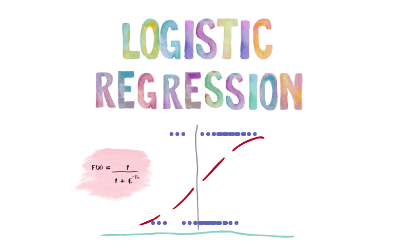
In logistic regression, we use the logistic function, which is defined as:
\[ \Large p(X) = \frac{e^{\beta_0 + \beta_1X}}{1 + e^{\beta_0 + \beta_1X}} \]
After a bit of manipulation of the above equation, we find that
\[ \Large \frac{p(X)}{1 - p(X)} = e^{\beta_0 + \beta_1X} \]
Whereas: \(p(X)/[1−p(X)]\): the odds, and can take on any value between 0 and .
By taking the logarithm of both sides of (4.3), we arrive at
\[ \Large log(\frac{p(X)}{1 - p(X)}) = \beta_0 + \beta_1X \]
Whereas:
- \(log(\frac{p(X)}{1 - p(X})\): the _log odds or logit.
In a logistic regression model, increasing \(X\) by one unit changes the log odds by \(\beta_1\).
9.2 Estimating the Regression Coefficients
Although we could use (non-linear) least squares to fit the model, the more general method of maximum likelihood is preferred, since it has better statistical properties. In general, logistic regression and other models can be easily fit using statistical software such as R, and so we do not need to concern ourselves with the details of the maximum likelihood fitting procedure.
An explanation of Maximum Likelihood for Machine Learning can be found here:
| Coefficient | Std. error | z-statistic | p-value | |
|---|---|---|---|---|
| Intercept | −10.6513 | 0.3612 | −29.5 | <0.0001 |
| balance | 0.0055 | 0.0002 | 24.9 | <0.0001 |
Table above shows the coefficient estimates and related information that result from fitting a logistic regression model on the Default data in order to predict the probability of default=Yes using balance. We see that \(\hat\beta_1\) = 0.0055; this indicates that an increase in balance is associated with an increase in the probability of default. To be precise, a one-unit increase in balance is associated with an increase in the log odds of default by 0.0055 units.
9.3 Multiple Logistic Regression
We now consider the problem of predicting a binary response using multiple predictors. By analogy with the extension from simple to multiple linear regression in Chapter 3, we can generalize the logistics regression formula as follows:
\[ \Large p(X) = \frac{e^{\beta_0+\beta_1X_1+...+\beta_pX_p}}{1+e^{\beta_0+\beta_1X_1+...+\beta_pX_p}} \]
9.4 Multinomial Logistic Regression
We sometimes wish to classify a response variable that has more than two classes. However, the logistic regression approach that we have seen in this section only allows for K = 2 classes for the response variable.
It turns out that it is possible to extend the two-class logistic regression approach to the setting of \(K > 2\) classes. This extension is sometimes known as multinomial logistic regression.