
Section 12 Generalized Linear Model
12.1 Overview
In reality, we may sometimes be faced with situations in which \(Y\) is neither qualitative nor quantitative, and so neither linear regression nor the classification approaches covered in this chapter is applicable.
To overcome the inadequacies of linear regression for analyzing the Bikeshare data set, we will make use of an alternative approach, called Poisson regression.
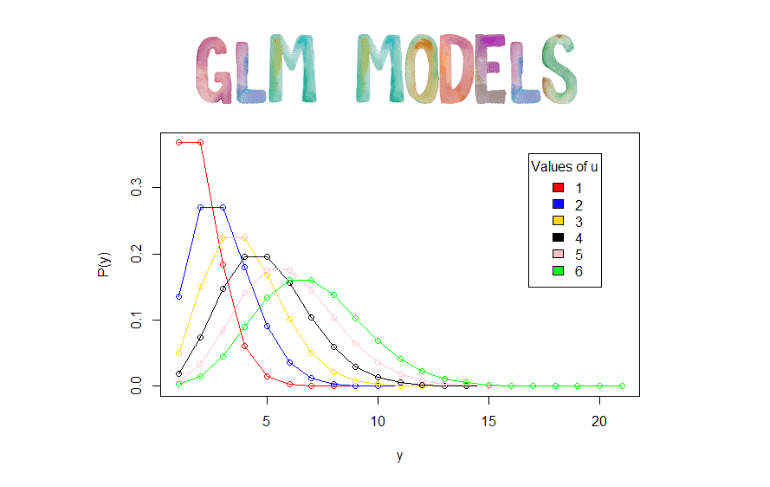
The Poisson distribution: is typically used to model counts; this is a natural choice for a number of reasons, including the fact that counts, like the Poisson distribution, take on nonnegative integer values.
Some important distinctions between the Poisson regression model and the linear regression model are as follows:
- Interpretation: To interpret the coefficients in the Poisson regression model, we must pay close attention to (4.37), which states that an increase in \(X_j\) by one unit is associated with a change in \(E(Y)\) = \(\lambda\) by a factor of exp(\(\beta_j\)). For example, a change in weather from clear to cloudy skies is associated with a change in mean bike usage by a factor of exp(−0.08) = 0.923, i.e. on average, only 92.3% as many people will use bikes when it is cloudy relative to when it is clear.
If the weather worsens further and it begins to rain, then the mean bike usage will further change by a factor of exp(−0.5) = 0.607, i.e. on average only 60.7% as many people will use bikes when it is rainy relative to when it is cloudy.
Mean-variance relationship: by modeling the data set with a Poisson regression, we implicitly assume that mean output in a given factor equals the variance of output to that variable. By contrast, under a linear regression model, the variance of the output always takes on a constant value. Thus, the Poisson regression model is able to handle the mean-variance relationship seen in the data set in a way that the linear regression model is not
nonnegative fitted values: There are no negative predictions using the Poisson regression model. This is because the Poisson model itself only allows for nonnegative values.
12.2 Generalized Linear Models in Greater Generality
We have now discussed three types of regression models: linear, logistic and Poisson. These approaches share some common characteristics:
Each approach uses predictors \(X_1,...,X_p\) to predict a response \(Y\). We assume that, conditional on \(X_1,...,X_p\), \(Y\) belongs to a certain family of distributions:
- For linear regression, we typically assume that \(Y\) follows a Gaussian or normal distribution.
- For logistic regression, we assume that \(Y\) follows a Bernoulli distribution.
- For Poisson regression, we assume that \(Y\) follows a Poisson distribution.
Each approach models the mean of \(Y\) as a function of the predictors:
- In linear regression, the mean of \(Y\) takes the form:
\[ E(Y|X_1, . . . ,X_p) = \beta_0 + \beta_1X_1 + · · · + \beta_pX_p \]
For logistic regression, the mean instead takes the form: \[ E(Y|X_1, . . . ,X_p) = Pr(Y=1|X_1, . . . ,X_p) \]
For Poisson regression, the mean takes the form: \[ E(Y|X_1, . . . ,X_p) = \lambda(X_1, . . . ,X_p) \]
The Gaussian, Bernoulli and Poisson distributions are all members of a wider class of distributions, known as the exponential family.
Other wellexponential known members of this family are the exponential distribution, the Gamma distribution, and the negative binomial distribution (which is not cover in this secion).
In general, we can perform a regression by modeling the response \(Y\) as coming from a particular member of the exponential family, and then transforming the mean of the response so that the transformed mean is a linear function of the predictors Poisson.
Any regression approach that follows this very general recipe is known as a generalized linear model (GLM). Thus, linear regression, logistic generalized linear model regression, and Poisson regression are three examples of GLMs.